Building a Performant Compiler from Scratch
Architecture, algorithms, and optimization techniques behind a 10k+ line compiler pipeline that lowers a C-like language to x86-64.

Introduction
I built a compiler that translates a C-like language called LB all the way down to x86-64 assembly, producing executables that can run directly on modern processors. The system consists of more than 10,000 lines of code and implements many of the classic components of a modern compiler, including instruction selection, register allocation, data-flow analysis, and multiple optimization passes.
Rather than implementing a single monolithic compiler, the system is structured as a pipeline of compilers. A program begins in the LB language and is successively translated through a sequence of intermediate languages. Each stage removes a layer of abstraction and enforces stronger invariants on the program representation. Early stages eliminate high-level constructs such as nested scopes and structured control flow. Later stages perform program optimizations, select machine-like instructions, and allocate hardware registers. By the time the program reaches the final stage, it is translated into x86-64 assembly, which is then assembled into machine code and linked with the runtime to produce the final executable.
This article is a technical deep dive into the system I built. It explores:
- the architecture of the compiler pipeline
- the core algorithms used inside the compiler
- how the system generates efficient machine code
- the challenges of debugging complex systems
Compiler Pipeline Architecture
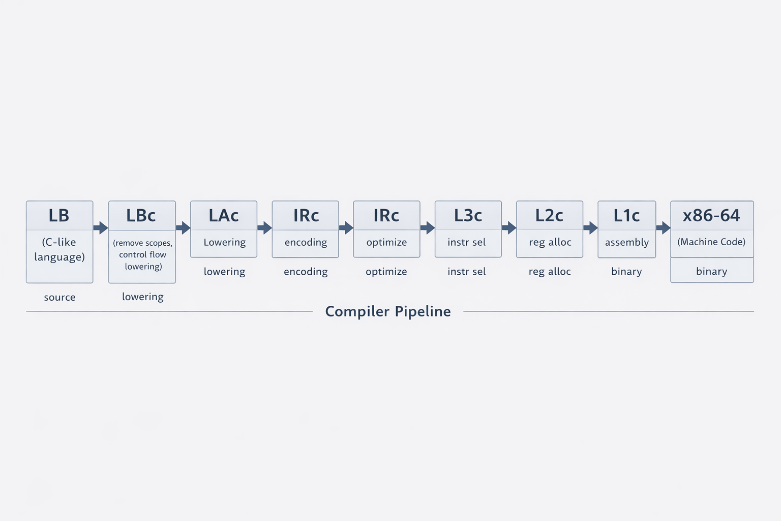
The compiler pipeline operates on seven languages: LB, LA, IR, L3, L2, L1, and x86-64. Each language has its own grammar, which can be found in the project repository. LB begins as a relatively abstract, C-like language. Each subsequent language becomes progressively closer to assembly and explicit register operations. This gradual reduction of abstraction is known as lowering.
The pipeline itself consists of six compilers: LBc, LAc, IRc, L3c, L2c, and L1c. Each compiler translates a program from one language into the next lower-level language. LBc translates LB code into LA code, LAc translates LA code into IR code, IRc translates IR code into L3 code, and so on until the program is eventually expressed as x86-64 assembly.
Each stage performs a well-defined transformation:
- LBc removes nested scopes, translates
ifandwhilestatements, and separates variable declarations that appear on the same line. - LAc encodes values and inserts checks for array accesses.
- IRc performs program optimizations and linearizes multi-dimensional arrays.
- L3c performs instruction selection, mapping higher-level operations to lower-level instructions.
- L2c allocates variables to hardware registers.
- L1c translates the L1 language into x86-64 assembly.
Once x86-64 assembly is produced, the program is assembled into machine code using an assembler and then linked with the runtime using a linker to produce the final executable.
To illustrate how the pipeline progressively lowers a program, consider the following simple LB program.
int64 main ( ){
  int64 v1, v2, v3
  v1 <- 1
  v2 <- 2
  v3 <- v1 + v2
  return v3
}After passing through the LBc compiler, variable declarations that originally appeared on the same line are separated and the program structure is simplified.
int64 main() {
  int64 v1_0
  int64 v2_0
  int64 v3_0
  v1_0 <- 1
  v2_0 <- 2
  v3_0 <- v1_0 + v2_0
  return v3_0
}Passing the program through LAc, we begin to see value encoding introduced.
define int64 @main () {
  :beginning_label
  int64 %v1_0
  %v1_0 <- 1
  int64 %v2_0
  %v2_0 <- 1
  int64 %v3_0
  %v3_0 <- 1
  %v1_0 <- 3
  %v2_0 <- 5
  int64 %new_var_0
  %new_var_0 <- %v1_0 >> 1
  int64 %new_var_1
  %new_var_1 <- %v2_0 >> 1
  int64 %new_var_2
  %new_var_2 <- %new_var_0 + %new_var_1
  %v3_0 <- %new_var_2 << 1
  %v3_0 <- %v3_0 + 1
  return %v3_0
}After passing through IRc, the number of lines of code becomes significantly smaller. This occurs because the IR compiler performs several optimizations. Notice that the program now returns 7 instead of 3. This is due to the value encoding scheme used in later stages of the compiler. In this representation, the least significant bit is set to 1 when the value represents an integer. Therefore, the integer 3 (binary 011) becomes the encoded value 111, which corresponds to 7.
define @main () {
  :beginning_label
  return 7
}Passing the program through L3c, we see that the return value is now stored in the register rax. This occurs because the L3c compiler enforces the system's calling convention, where the callee places the return value in rax before returning control to the caller.
(@main
  (@main 0
    :__label__0
    rax <- 7
    return
  )
)Passing the L3 program through L2c, we observe relatively few changes. This is because the example program does not use many variables. In general, the L2c compiler replaces program variables with hardware registers through register allocation.
(@main
  (@main
    0 0
    :__label__0
    rax <- 7
    return
  )
)Finally, the L1c compiler translates the L1 program into x86-64 assembly instructions.
.text
.globl go

go:
  # save callee-saved registers
  pushq %rbx
  pushq %rbp
  pushq %r12
  pushq %r13
  pushq %r14
  pushq %r15

  call _main

  # restore callee-saved registers and return
  popq %r15
  popq %r14
  popq %r13
  popq %r12
  popq %rbp
  popq %rbx
  retq

_main:
___label__0:
  movq $7, %rax
retqThrough this example, we can see how a high-level program is gradually transformed and optimized as it moves through the compiler pipeline, eventually becoming executable machine code.
Why Use Multiple Stages?
An intentional design decision was to avoid lowering programs directly from LB to x86-64. Instead, the compiler is structured as a sequence of smaller compilers, each responsible for removing a specific layer of abstraction. This allows the complexity of the system to be tackled piece by piece. A single monolithic compiler would have to handle all transformations at once, making the system significantly harder to implement and reason about.
This separation is also extremely helpful when debugging the compiler itself. If a program fails during compilation or produces incorrect output, I can inspect the intermediate languages produced at each stage to determine where an invariant was violated. Because each stage has clearly defined assumptions about its input, it becomes much easier to isolate and diagnose errors.
The modular design also mirrors the architecture of modern compilers such as LLVM, which
rely heavily on intermediate representations and staged lowering. If there are n
high-level source languages and m target architectures, compiling each source directly
to each architecture requires n x m separate compilers. Introducing a shared
intermediate representation reduces that to n + m components: n frontends and
m
backends.
Register Allocation
A key part of the L2c compiler is register allocation. Most programming languages allow the use of a theoretically unlimited number of variables, but the hardware provides only a limited number of registers. The compiler must therefore decide which variables reside in hardware registers and which must temporarily be stored in memory.
To solve this problem, the compiler uses the Chaitin-Briggs register allocation algorithm, a graph-coloring approach that models register assignment as a graph coloring problem over variable interference. By analyzing where variables are simultaneously live, the compiler constructs an interference graph and attempts to assign each variable a register without conflicts. When this is not possible, some variables are spilled to memory.
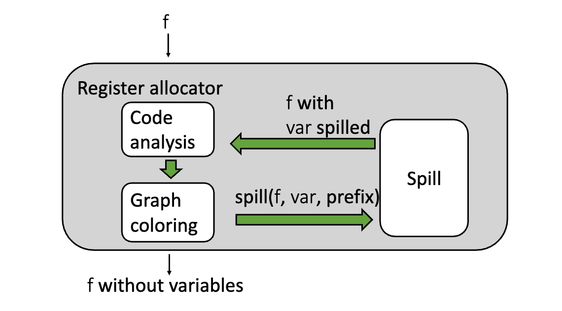
To determine which variables may share registers, the compiler first performs liveness analysis. For every instruction in the program, the compiler computes which variables are live immediately before and immediately after that instruction. A variable is live at a point if its current value may still be used in the future before being overwritten.
Using the results of liveness analysis, the compiler constructs an interference graph. In this graph, each node represents a variable, and an edge between two nodes indicates that the corresponding variables are live at the same time and therefore cannot share a register.
Once the interference graph is built, register allocation becomes a graph coloring problem. Each hardware register is treated as a color, and the goal is to assign a color to every node in the graph such that no two adjacent nodes share the same color. If the graph can be colored using the available registers, the compiler has successfully mapped variables to hardware registers.
When the graph cannot be colored with the available number of registers, the compiler must spill one or more variables. Spilling rewrites the program by storing those variables in memory and inserting load and store instructions around their uses. After spilling, the compiler recomputes liveness, rebuilds the interference graph, and attempts to color it again. This process repeats until a valid coloring is found.
Ultimately, register allocation reconciles abstraction with hardware limitations. While the L2 language provides the illusion of unlimited variables, the L1 language must operate within the finite set of physical registers available on the processor.
Instruction Selection
A central component of the L3c compiler is instruction selection: choosing which lower-level instructions to use when translating higher-level operations. A naive approach would translate L3 instructions one by one, independent of surrounding context. While correct, that often produces inefficient code.
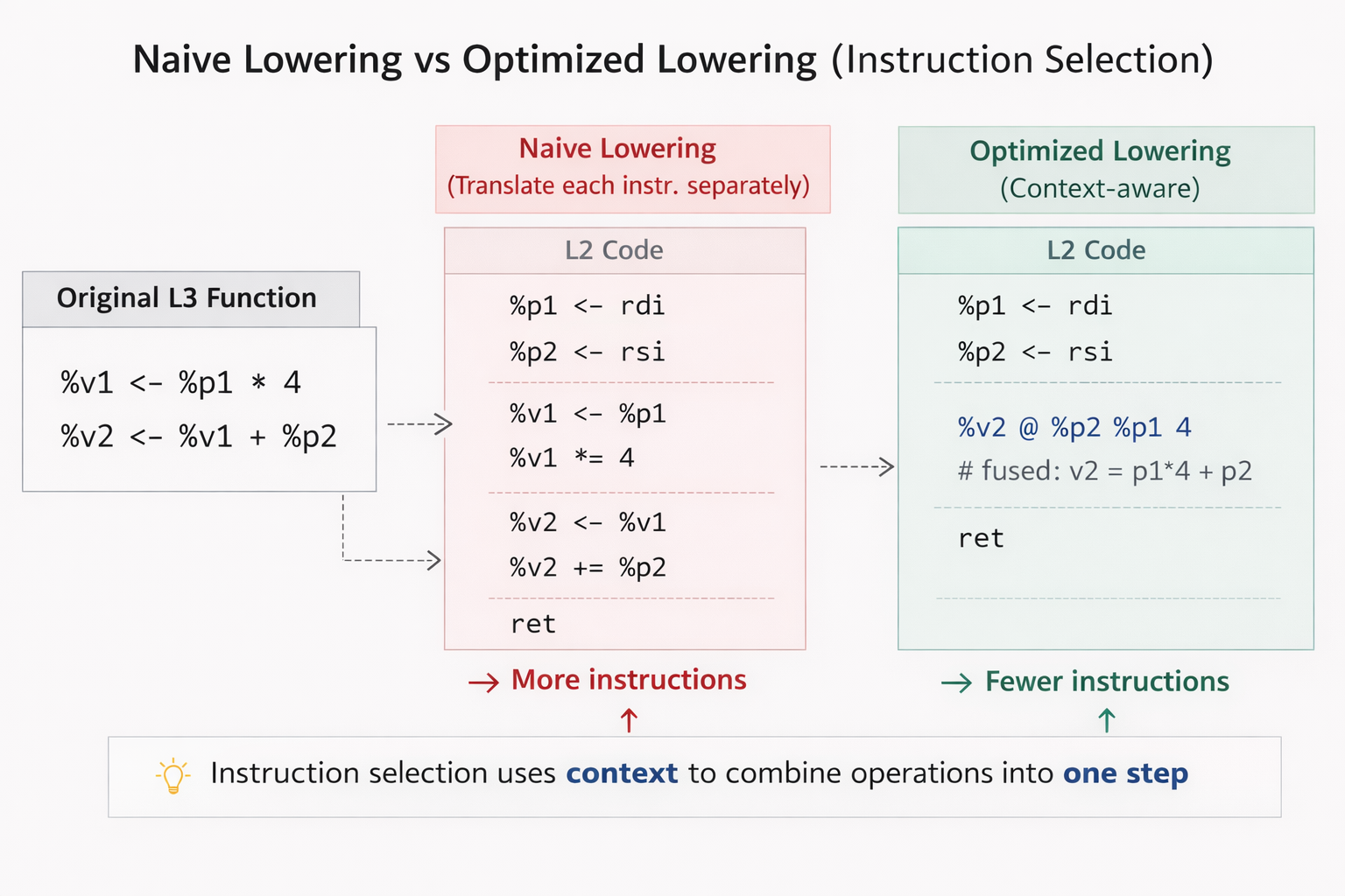
To exploit larger optimization opportunities, the compiler represents instructions as trees. A tree describes the computation performed by an instruction in terms of operators and operands. When it is safe to do so, these trees can be merged, exposing larger computation patterns that span multiple instructions.
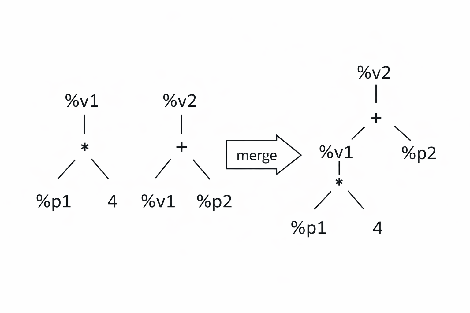
After constructing these trees, the compiler performs tiling. A tile is a pattern that matches a subtree and specifies how that pattern should be translated into L2 instructions. Each tile has an associated cost equal to the number of L2 instructions it generates. The objective is to cover the entire tree with tiles such that the total cost is minimized.
Computing the globally optimal tiling is expensive, so the compiler uses a greedy heuristic called maximal munch. Starting from the root of the tree, the algorithm selects the largest tile that matches the current subtree. If multiple tiles match, the tie is broken using the tile with the lowest cost. The algorithm then recursively applies the same rule to the remaining subtrees.
Maximal munch does not guarantee a globally optimal tiling, but it is simple, efficient, and performs well in practice for real instruction sets.
Benchmarking
The first goal of any compiler is correctness: the generated program must behave exactly as intended. Once correctness is achieved, the next objective is performance. To evaluate that performance, I built a benchmark harness that measures the runtime of compiled programs in a controlled and repeatable way.
The harness performs several tasks:
- verifies the program output against an oracle
- runs a configurable number of warmup executions
- runs a configurable number of measured repetitions
- records average, median, minimum, and maximum runtime in milliseconds
- emits results in CSV format for later analysis
Warmup runs help stabilize performance by warming instruction caches, data caches, and branch predictors. After the warmup phase, the harness measures repeated executions and records the results in CSV format so optimizations can be compared consistently over time.
Optimizations
With the benchmark harness in place, I implemented and measured a range of optimizations. The system includes:
- constant propagation
- dead code elimination
- constant folding
- branch simplification
- unreachable basic block removal
- redundant LA bounds and null-check elimination
- reuse of decoded integer values across LA lowering chains
In the following sections, I focus on constant propagation and how it unlocks other optimizations such as dead code elimination and constant folding.
Constant Propagation
When evaluating the performance of compiled programs, we ultimately care about wall-clock time. During development, though, compilers often use instruction count as a rough proxy for performance. In general, programs that execute fewer instructions tend to run faster.
Consider the following program:
b <- 2
c <- b + 4
d <- c * 8
return d
Since the value of b is known to be the constant 2, the compiler can substitute that
value directly into later expressions. This is constant propagation:
b <- 2
c <- 2 + 4
d <- c * 8
return d
Once constants appear inside algebraic expressions, the compiler can evaluate them at compile time, a process known as constant folding:
b <- 2
c <- 6
d <- c * 8
return d
Propagating one step further gives:
b <- 2
c <- 6
d <- 6 * 8
return d
A final constant folding operation yields:
b <- 2
c <- 6
d <- 48
return d
At this point, the assignments to b and c are no longer needed. Dead code
elimination removes them:
d <- 48
return d
Through a few rounds of simple optimizations, the program is reduced from four instructions down to two instructions.
Optimization Results
To evaluate the impact of the implemented optimizations, I benchmarked the generated executable using a matrix-multiplication workload. This program performs a large number of arithmetic operations and serves as a useful stress test for the quality of the generated machine code.
Before applying any optimizations, the compiled program ran in 24,960 ms on average. After enabling the optimization passes, the average runtime decreased to 5,369 ms. That corresponds to a 4.65x speedup, reducing total execution time by approximately 78.5%.
| Configuration | Average Runtime |
|---|---|
| No optimizations | 24,960 ms |
| With optimizations | 5,369 ms |
These benchmarks were run on 2× Intel Xeon Gold 6126 @ 2.60 GHz (24 physical cores, 48 hardware threads total) with 251 GiB RAM, running Red Hat Enterprise Linux 8.10 on Linux 4.18.0-553.107.1.el8_10.x86_64.
Debugging a Multi-stage Compiler
Debugging a multi-stage compiler pipeline is difficult because a failure observed at one stage does not necessarily originate there. A program passes through several compilers before producing an executable, so the root cause may lie anywhere earlier in the pipeline.
Another complication is that most intermediate languages in the pipeline are not executable. Only the final x86-64 binary can actually be run. Debugging therefore requires inspecting the intermediate programs produced by each compiler stage and determining where the first incorrect transformation occurs.
I ran into a concrete example of this while implementing the LAc compiler. One of its
responsibilities is value encoding. Because encoding operations require intermediate
computations, the compiler needs to introduce temporary variables. My initial
implementation generated names such as newVar0, newVar1, and so on using a global
counter.
int64 %new_var0
%new_var0 <- %v1_0 >> 1
int64 %new_var1
%new_var1 <- %v2_0 >> 1
int64 %new_var2
%new_var2 <- %new_var0 + %new_var1
%v3_0 <- %new_var2 << 1
%v3_0 <- %v3_0 + 1prog.IR.An issue surfaced while running a Fibonacci test case. Instead of producing the expected sequence of numbers, the output values were extremely large.
The first hypothesis was integer overflow. Since Fibonacci numbers grow quickly, it was plausible that somewhere in the pipeline 32-bit integers were being used instead of 64-bit integers. Investigation did reveal several locations where integers were incorrectly handled as 4-byte values, but correcting these issues did not resolve the test failure. This was expected in hindsight because the test case only computed the first few Fibonacci numbers, which are too small to overflow a 64-bit integer.
Instead of continuing to guess possible causes across the pipeline, the next step was to determine where the incorrect values first appeared.
Because the intermediate languages are not executable, this required inspecting the code generated at each stage of the pipeline. By tracing the program through the intermediate outputs, the values first became incorrect in the L3 code.
This narrowed the problem to the stages responsible for producing that code. The IRc compiler translates IR code into L3 code, so the L3 program depends on two things: the IR program produced by the LAc compiler and the logic inside the IRc compiler.
If the L3 code is incorrect, then one of the following must be true:
- The IR program produced by LAc is correct, but the IRc compiler introduced an error during translation.
- The IR program produced by LAc is already incorrect, so the IRc compiler is translating faulty input.
- Both stages contain errors.
This reduced the debugging scope to the LAc and IRc compilers.
Inspecting the IR output produced by the LAc compiler revealed the issue. When the LAc
compiler generated temporary variables during value encoding, it created names such as
newVar0. One of the test programs already used a variable with that name. This
caused a variable name collision, which corrupted intermediate values and resulted in the
incorrect Fibonacci output.
To fix this, the compiler now guarantees that every compiler-generated temporary has a fresh name. Before inserting a temporary, the compiler checks whether that name is already used anywhere in the function. If it is, the compiler increments a function-scoped counter, generates a different candidate name, and repeats the check until it finds one that is unique. This prevents compiler-generated temporaries from colliding with user-defined variables or previously generated temporaries.
Conclusion
This compiler translates programs through a sequence of intermediate languages, from LB and LA down to IR, L3, L2, L1, and finally x86-64 assembly. Early stages remove high-level abstractions. Later stages perform optimizations, select lower-level instructions, and allocate hardware registers.
Along the way, the implementation relies on several core compiler techniques, including tree-tiling-based instruction selection, interference-graph-based register allocation, and data-flow-driven optimizations such as constant propagation and dead code elimination.
The result is a complete compiler pipeline that lowers high-level programs into efficient executable machine code.
Check out the repo here!
This project was developed in Northwestern's CS 322 compilers course. The course provided the language specifications, test cases, and runtime, while the compiler implementations themselves were built from the ground up.